[ML]机器学习和Python实践(二)决策树(中)

在前面已经介绍了决策树,由于篇幅限制,我们在选择最好的数据方式那就草草了事。现在,我们开始了下一篇。

1
2
3
4
5
6
7
8
9
10
11
12
13
14
15
16
17
18
def chooseBestFeatureToSpilt(dataSet) :
numFeatures = len(dataSet[0])-1
baseEntropy = calcShannonEnt(dataSet)
bestInfoGain = 0.0
bestFeature = -1
for i in range(numFeatures) :
featList = [example[i] for example in dataSet] # 创建唯一的分类标签列表
uniqueVals = set(featlist)
newEntropy = 0.0
for value in uniqueVals :
subDataSet = spiltDataSet(dataSet, i, value) # 计算每一种划分方式的信息熵
prob = len(subDataSet)/float(len(dataSet))
newEntropy += prob*calcShannonEnt(subDataSet)
infoGain = baseEntropy - newEntropy
if infoGain>baseEntropy : # 计算最好的信息增益
bestInfoGain = infoGain
bestFeature = i
return bestFeature

函数chooseBestFeatureToSplit使用了前面两者的函数。数据需要满足以下要求:1.数据必须由列表元素主城的列表,而且所有的列表元素都具有相同的数据长度;2.数据的最后一列或者每个实例的最后元素是当前实例的类别标签。数据集的第一行就能判定当前实例的类别标签。

在开始划分数据集之前,程序清单第三行代码计算了整个数据集的原始香农熵,我们应当保存最初的无序度量值,用于与划分完成之后的数据集的熵值进行比较。第一个for循环遍历了数据集中的所有特征。使用列表推导来创建心得列表,将数据集中的所有第i个特征值或者所有可能存在的值写入这个新的list中,然后使用Python原生的集合(set)数据类型。这个数据类型和list相似,但是key互不相同。这个数据类型非常类似于数学中的集合。

而我们运行了以下代码之后,发现了我们所划分的区域处于0。

1
2
3
4
if __name__ =="__main__":
myData,labels = createDataSet()
print chooseBestFeatureToSpilt(myData)
print myData

而结果为:

1
2
0
[['1', '1', 'yes'], ['1', '1', 'yes'], ['1', '0', 'no'], ['0', '1', 'no'], ['0', '1', 'no']]

也就是说,第0特征是最适合划分数据集的特征。按照这种方式划分数据集,也就是说第0特征为1的放在一个组,为0放在另一个组,这样与原数据比起来,确实是一种很好的划分数据的方式,只有一个被误判了,同样的,我们可以计算香农熵,其结果也能符合要求。(表见上的博客)

1.递归构建决策树

1.1原理

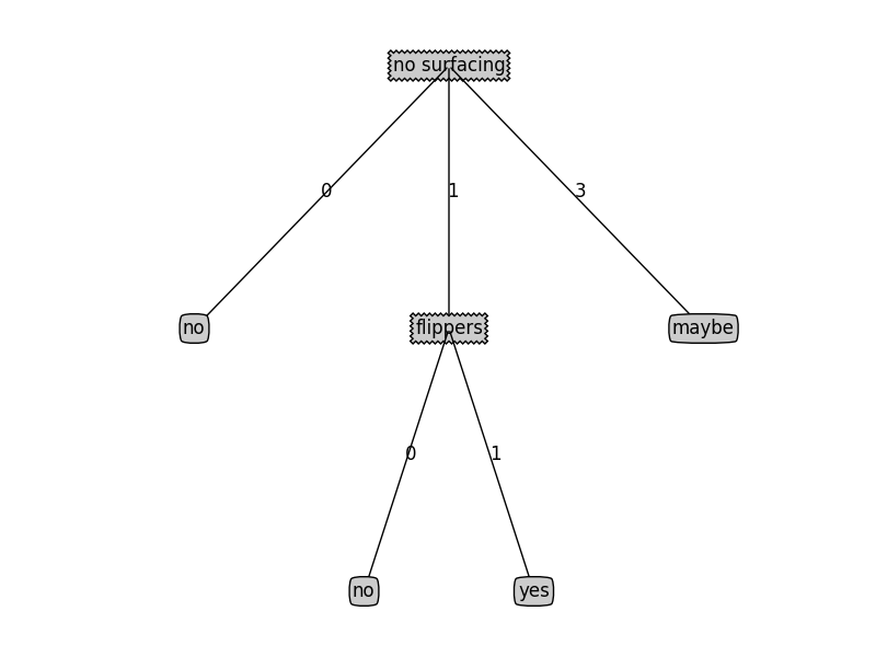
首先得到原始数据集,然后基于最好的属性值划分数据集,当特征值多于两个的时候,就需要进行大于两个分支的数据集划分。当进行了第一次划分之后,数据会被向下传递至树分支的下一个节点,然后进行递归的划分数据。

这里,我们再一次引用开始的图片来表示我们的递归划分的过程。

[caption id=”attachment_430” align=”aligncenter” width=”573”]决策树 来源:百度百科[/caption]

但是和DFS一样,我么必须知道什么时候递归结束。当程序遍历完所有划分的数据集的属性或者每个分支下的所有实例都具有相同的分类的时候所得到的叶子节点或者终止块。任何到达叶子节点的数据必然属于叶子节点的分类

注意了,我们可以设置算法可以划分的最大分组数目,这也涉及到其他决策树的算法,例如C4.5和CART,但是需要指出的是,这些算法在运行的时候并不是总是在每次划分分组的时候都能够消耗特征,正是因为此,这些算法可能在实际的问题上引发一些问题。

所以我们似乎需要使用函数来表达字典来辅助我们建立决策树:

1
2
3
4
5
6
7
8
9
10
import operator
def majorityCnt(classList):
classCount = {}
for vote in classList:
if vote not in classCount.keys():
classCount[vote]=0
classCount[vote] +=1 # 创建键值为classList中唯一值得数据字典,统计每个标签出现的频率
sortedClassCount = sorted(classCount.iteritems(),key=operator.itemgetter(1),reversed=True)
return sortedClassCount[0][0]

1.2创建决策树

程序使用了两个参数,数据集和标签列表。标签列表中包含了数据集中所有特征的标签,这个是作为给出数据明确的含义。

1
2
3
4
5
6
7
8
9
10
11
12
13
14
15
16
def createTree(dataSet,labels):
classList = [example[-1] for example in dataSet] #创建包含数据集中所有类的标签
if classList.count(classList[0]) == len(classList):
return classList[0] #类别相同就停止继续划分
if len(dataSet[0]) ==1:
return majorityCnt(classList) #遍历完所有特征时返回出现次数最多的
bestFeat = chooseBestFeatureToSpilt(dataSet)
bestFeatLabel = labels[bestFeat]
myTree = {bestFeatLabel:{}}
del(labels[bestFeat])
featValues = [example[bestFeat] for example in dataSet]
uniqueVals = set(featValues) #得到所有的属性值
for value in uniqueVals:
subLabels = labels[:]
myTree[bestFeatLabel][value] = createTree(splitDataSet(dataSet,bestFeat,value),subLabels)#递归过程
return myTree

字典myTree储存了树的所有信息,这对于绘制其后的树形图十分重要。当前数据集选取最好的特征存储在bestFeat中,得到了列表包含的所有属性值。而在最后,遍历当前选择特征所包含的所有的属性值,在每个数据集划分上递归调用函数createTree(),得到的返回值将被插入到字典变量myTree中,因此函数终止执行时,字典将会嵌套很多代表叶子节点信息的字典数据。而在循环的第一行,sublabels = labels[:],其深复制了类标签,并且将其储存于新列表之中,使用sublabels代替原始列表。

当然,我们也用了下面来表示这个过程。

1
2
3
4
5
6
if __name__ =="__main__":
myData,labels = createDataSet()
print chooseBestFeatureToSpilt(myData)
print myData
myTree = createTree(myData,labels)
print myTree

结果我们也给出来了:

1
2
3
0
[['1', '1', 'yes'], ['1', '1', 'yes'], ['1', '0', 'no'], ['0', '1', 'no'], ['0', '1', 'no']]
{'no surfacing': {'1': {'flippers': {'1': 'yes', '0': 'no'}}, '0': 'no'}}

2.使用Python的matplotlib注解绘制树形图

2.1Matplotlib注解

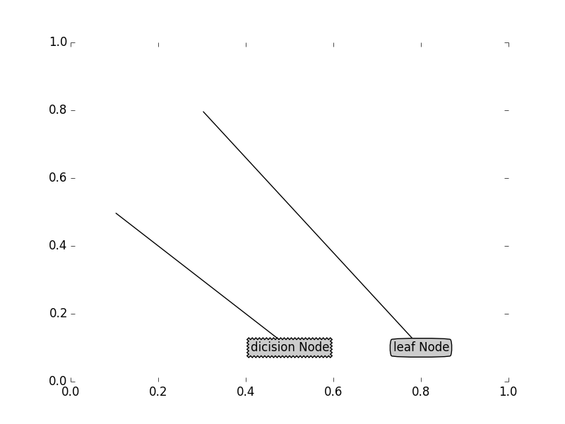
matplotlib提供了一个注解工具annotations,他可以在数据图形上添加文本注释,可以用于解释数据内容,而且工具内嵌支持带箭头的划线工具。

1
2
3
4
5
6
7
8
9
10
11
12
13
14
15
16
17
18
19
# -*- coding: UTF-8 -*-
__author__ = 'kidozh'
import matplotlib.pyplot as plt
decisonNode = dict(boxstyle="sawtooth",fc="0.8") # 定义箭头和文本框
leafNode = dict(boxstyle="round4",fc="0.8")
arrow_args = dict(arrowstyle="<-")
def plotNode(nodeTxt,centerPt,parentPt,nodeType): #绘制带有箭头的注释
createPlot.axl.annotate(nodeTxt,xy=parentPt,xycoords='axes fraction',xytext=centerPt,textcoords='axes fraction',va="center",ha="center",bbox=nodeType,arrowprops=arrow_args)
def createPlot():
fig = plt.figure(1,facecolor='white')
fig.clf()
createPlot.axl = plt.subplot(111,frameon=False)
plotNode(u'dicision Node',(0.5,0.1),(0.1,0.5),decisonNode)
plotNode(u'leaf Node',(0.8,0.1),(0.3,0.8),leafNode)
plt.show()

figure_1

知道如何构造注解树之后,我们必须明晰树究竟有多少个叶节点(也就是X轴的长度),也应该知道树有多少层,一边可以正确确定y轴高度,这里就需要定义两个函数分别获得叶节点数目和层数

1
2
3
4
5
6
7
8
9
10
11
12
13
14
15
16
17
18
19
20
21
22
def getNumLeafs(myTree):
numLeafs = 0
firstStr = myTree.keys()[0]
secondDict = myTree[firstStr]
for key in secondDict.keys():
if type(secondDict[key]).__name__=='dict':#如果是字典就加上之后的结果
numLeafs+=getNumLeafs(secondDict[key])
else:
numLeafs+=1
def getTreeDepth(myTree):
maxDepth = 0
firstStr = myTree.keys()[0]
secondDict = myTree[firstStr]
for key in secondDict.keys():
if type(secondDict[key]).__name__ =='dict':
thisDepth = 1+getTreeDepth(secondDict[key])
else:
thisDepth = 1
if thisDepth>maxDepth:
maxDepth = thisDepth
return maxDepth

上述函数具有两个相同的结构,后面我们也会用到这两个函数,为了节省时间,我也写了个函数预先存储树的信息,避免每次测试代码时都需要从数据中创建树的麻烦

1
2
3
4
5
6
7
8
def retrieveTree(i):
listOfTrees=[{'no surfacing':{0:'no',1:{
'flippers':{0:'no',1:'yes'}}}},
{'no surfacing':{0:'no',1:{
'flippers':{0:{'head':{0:'no',1:'yes'}},1:'no'}}}}
]
return listOfTrees[i]

现在可以将前面的函数组成到一起,如下:

1
2
3
4
5
6
7
8
9
10
11
12
13
14
15
16
17
18
19
20
21
22
23
24
25
26
27
28
29
30
31
32
33
34
def plotMidText(cntrPt,parentPt,txtString):
xMid = (parentPt[0]-cntrPt[0])/2.0+cntrPt[0] # 在父子节点之间填充文本信息
yMid = (parentPt[1]-cntrPt[1])/2.0+cntrPt[1]
createPlot.ax1.text(xMid,yMid,txtString)
def plotTree(myTree,parentPt,nodeTxt):
numLeafs = getNumLeafs(myTree) #计算宽与高
depth = getTreeDepth(myTree)
firstStr = myTree.keys()[0]
cntrPt = (plotTree.xOff+(1.0+float(numLeafs))/2.0/plotTree.totalW,plotTree.yOff)
plotMidText(cntrPt,parentPt,nodeTxt)
plotNode(firstStr,cntrPt,parentPt,decisonNode) #标记子节点属性
secondDict = myTree[firstStr]
plotTree.yOff = plotTree.yOff-1.0/plotTree.totalD # 减少y偏移
for key in secondDict.keys():
if type(secondDict[key]).__name__ == 'dict':
plotTree(secondDict[key],cntrPt,str(key))
else:
plotTree.xOff = plotTree.xOff + 1.0/plotTree.totalW
plotNode(secondDict[key],(plotTree.xOff,plotTree.yOff),cntrPt,leafNode)
plotMidText((plotTree.xOff,plotTree.yOff),cntrPt,str(key))
plotTree.yOff = plotTree.yOff + 1.0/plotTree.totalD
def createPlot(inTree):
fig = plt.figure(1,facecolor='white')
fig.clf()
axprops = dict(xticks=[],yticks=[])
createPlot.ax1 = plt.subplot(111,frameon=False,**axprops)
plotTree.totalW = float(getNumLeafs(inTree))
plotTree.totalD = float(getTreeDepth(inTree))
plotTree.xOff = -0.5/plotTree.totalW
plotTree.yOff = 1.0
plotTree(inTree,(0.5,1.0),'Tree')
plt.show()

上面我们可以看到,全局变量plotTree.totalW存储树的宽度,而plotTree.totalD存储树的深度,利用这两个量就能保证树绘制在水平和垂直方向上的中心位置。而plotTree也是一个递归函数,树的宽度用于计算放置判断节点的位置,主要计算原则是将它放在所有叶子节点的中间,而plotTree.xOff和plotTree.yOff则用来追踪已经绘制的节点位置,以及放置这个节点的位置(绘图x和y轴的有效范围均是0~1)。

接着,画出子节点具有的特征值,或者沿此分支向下的数据实例必须有的特征值。使用plotMidText计算父子节点的中间位置,并且在此处添加简单的文本标签信息。

然后,按比例减少全局变量plotTree.yOff,并且标注此处将要画出的子节点,这些节点可以是子节点也可以是判定节点,这里仅需要保存绘制图形的轨迹,由于我们自顶而下的绘制图形,需要依次递减y坐标值,然后继续计算出子树的叶子结点数目和树的深度,递归的画下去,若节点是叶子结点,则在图形中画出叶子结点,若不是,则递归调用plotTree函数,绘制了所有的子节点之后,增加全局变量Y的偏移。

那么我们来试一下:

1
2
3
4
5
6
7
__author__ = 'kidozh'
# -*- coding: UTF-8 -*-
import decisionTree.treePlotter
myTree = decisionTree.treePlotter.retrieveTree(0)
myTree['no surfacing'][3] ='maybe'
decisionTree.treePlotter.createPlot(myTree)

结果如下:

figure_2